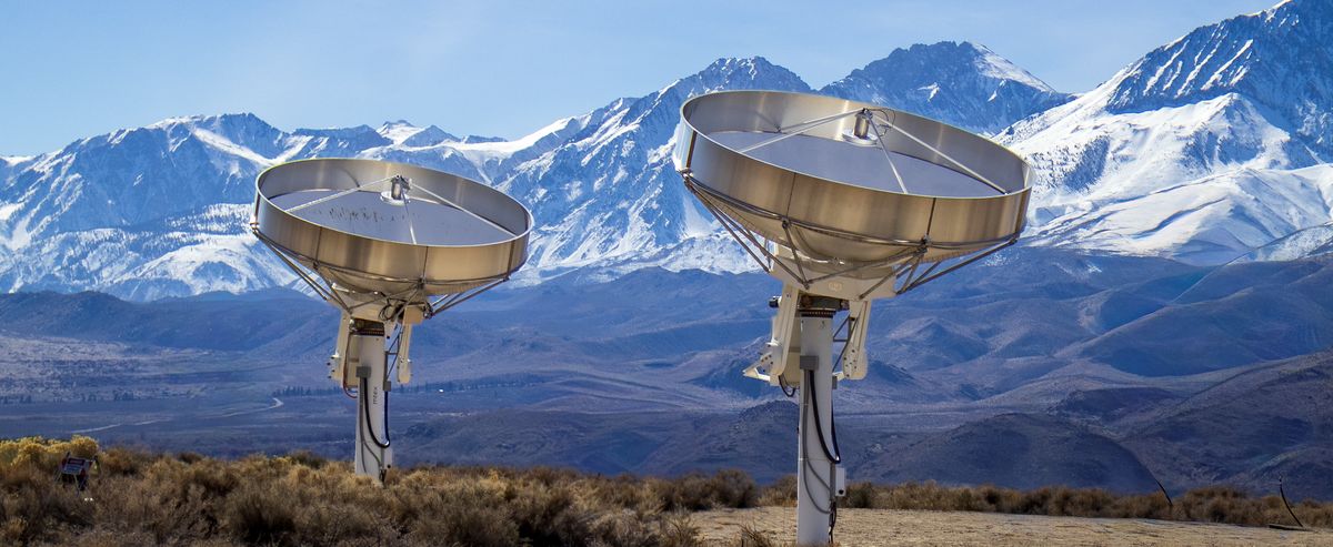
Two DSA prototype antennas in Owens Valley with the snow-covered Sierra Nevada behind them

DSA Sensitivity Calculator

Noise, resolution and detection limits for every DSA data product: continuum, HI, polarization, FRBs, pulsar searches and pulsar timing, for any position in the survey or a targeted observation.

1,650 × 6.15 m dishes0.7–2.0 GHzδ ≥ −30°, 30,940 deg²21-min pointings
DSA prototype antennas, Owens Valley Radio Observatory
Observation
Position (J2000)
Survey depth
Gaussian convolution, equivalent to a uv taper. Adds smoothed noise and brightness temperature for continuum, HI and polarization. 0 = native.
Data products
Advanced instrument & search settings
System
Targeted tracks
FRB search
Pulsar search
0 = whole pointing (Chronoscope design)
Pulsar timing reference MSP
Loading sky model and array configuration…

How the numbers are made

Every value comes from one noise model, implemented twice: in the browser (JavaScript) and as a Python package with identical results. Inputs are the FDR design documents, the antenna configuration and measured site data.

System temperature & SEFD

SEFD = 2k Tsys / (η A), A = π(6.155 m)²/4

  • Tsys = 21.4 K at zenith on cold sky, η = 0.67, flat across the band.
  • Spillover rises with zenith angle, from the Tsys/η table used in survey design (+10.6 K in Tsys/η at δ = −30°).
  • Galactic synchrotron from GSM2008, smoothed by the primary beam at each frequency and added above the median |b| > 30° sky. It reaches ~100 K at 0.7 GHz towards the Galactic Centre.
Thermal noise & mosaics

σ = SEFD / √(N(N−1) · 2 · Δνunflagged · teff)

  • Δνunflagged = ∫(1 − occupancy) dν from the selected RFI profile. The default, Spring Valley model extrapolated, keeps the measured frequency pattern but scales it to DSA sensitivity, as if each channel had 24× as many transmitters above the flagging threshold: 15% of the band is lost, against 2.8% in the measurement. The design documents assumed 65% usable; add 24% extra loss under Advanced to compare.
  • Survey mosaics: teff = 21 min × Z(ν) × Neff(ν). Z is the mean mosaic weight of the hexagonal grid (θhex = 1.667°, θrow = 1.45°): 5.35 at 0.7 GHz, 1.44 at 1.35 GHz, 0.66 at 2.0 GHz.
  • Neff averages the epochs of the tiles under the squared primary beam, so depth changes smoothly across tile boundaries and falls off at the southern edge (δ = −30.45°).
  • Targeted: primary-beam centre, 1/SEFD² weighted along the hour-angle track.

Resolution

  • Natural-weighted PSF from the dsa1650_P305_v2.5.6.8 configuration: 3.03″ (E–W) × 2.31″/cos ZA (N–S) at 1.35 GHz, scaling as 1/ν.
  • Hour-angle tracks average the projected snapshot PSFs, matching a full FFT of the uv coverage to ~1%.
  • Robust weighting changes beam and noise by the per-frequency factors in the Rosero confusion memo.
  • The full-band beam and effective frequency follow the window weights used to combine the ten 130-MHz images.

Confusion

σc = fβ(θ) · θ² · (ν / 1.4 GHz)−0.7

  • Condon's Universal Confusion Calculator with βmin = 16, digitized from the Rosero memo. It reproduces the memo's tables to within 1%.
  • Survey tiles use the imaging and summation weighting that gives the lowest total noise in their final coadd. Targeted observations do the same unless you choose one.
  • Continuum-subtracted HI, and Stokes Q, U and V, are not confusion limited.
  • Smoothed continuum: by default the sources above 5σ at full resolution are subtracted first. What remains is the Poisson noise of the fainter sources, σ² = Ωe ∫0Slim S² n(S) dS, with n(S) the counts behind the confusion curve. It grows only linearly with beam size, so its Tb falls with scale.

Smoothing = tapering

  • Convolving an image with a Gaussian of FWHM θ is equivalent to a Gaussian uv taper exp(−π²θ²|u|²/4 ln2).
  • The noise per smoothed beam rises by √⟨T²⟩/⟨T⟩ over the array's visibilities, because the taper down-weights the long baselines that carry most of the sensitivity. It uses the real configuration: every baseline shorter than 1 km (about 13,000 are shorter than 0.9 km, down to 10 m; the whole VLA has 351) and every 13th longer one.
  • The smoothed beam is taken as the requested Gaussian, as in a restored image. Tapering the dirty beam instead gives a main lobe within 2% of it up to 1′ and within 13% up to 10′ at 1.35 GHz. Beyond ~15′ (~30′ at 0.7 GHz) only a few dozen baselines contribute, and the beam comes out narrower with 10–40% sidelobes. Smoothed products assume natural weighting.

Time domain

  • FRBs: cross-correlation beams, 1 ms sampling, 122.7 kHz channels (DM smearing 8.3 μs · DM · ΔνMHz/νGHz³), bands at 930/1410/1800 MHz. Values are for a burst at a beam centre; beam-tiling losses are not included.
  • Pulsar search: radiometer equation with Weff = √(W² + tsamp² + tDM²). The blind search uses 11.9″ tapered beams (taper loss from the configuration); the targeted search uses full phased-array beams.
  • Pulsar timing: four phased-array beams, 0.7–2.0 GHz, coherent dedispersion, σTOA ≈ W50/(S/N).

Survey plan

The Cadenced All-Sky Survey has 5 × 12,850 = 64,250 pointings of 21 minutes. Epochs are assigned per 72.5 deg² tile of the tiered-tile scheme (429 tiles). Each plan below is scored with the noise model above, counting continuum sources above 5σ in the final full-band coadd.

v2-A is the default. It keeps the DSA-00264 depths: 7 epochs in the Euclid/HSC footprint, and in the Galactic plane and bulge for pulsar follow-up. The published Fig. 1 leaves 1,140 of the 64,250 pointings unused and sets the wide area by declination alone; v2-A uses them all, placing the wide-area epochs where they add the most 5σ detections, with at least 2 everywhere.

The instrument

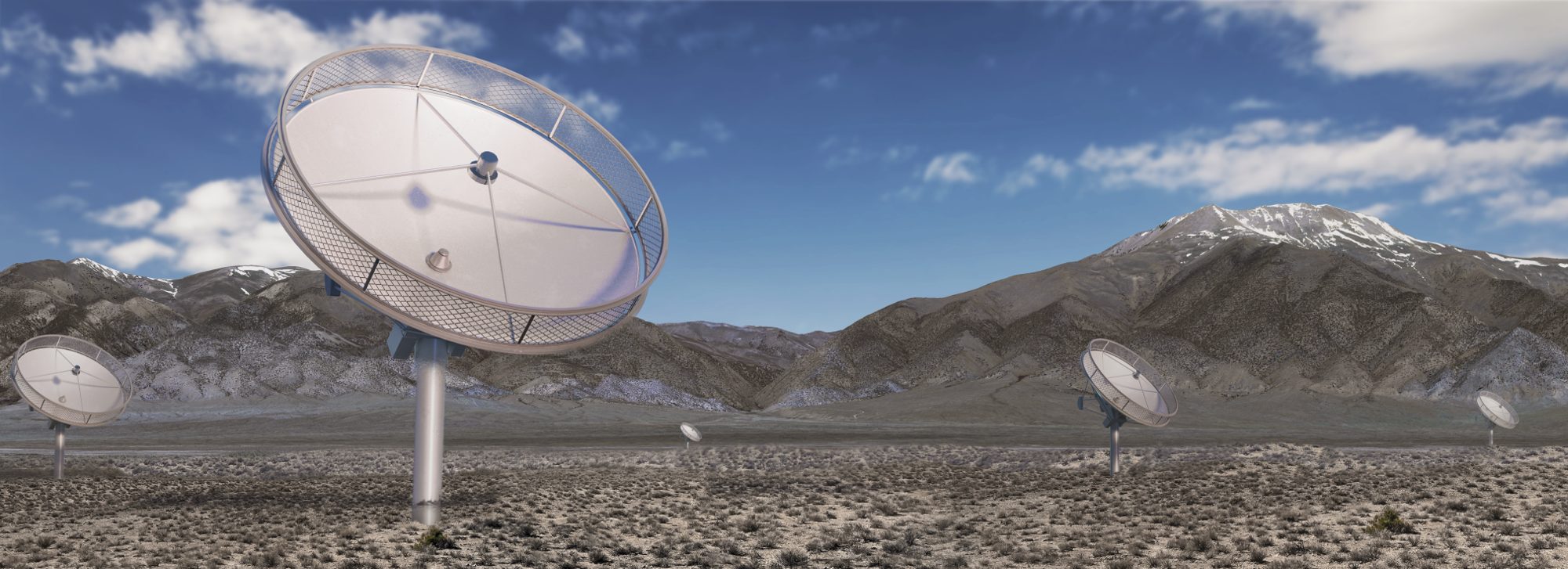
Rendering of DSA antennas on a sagebrush valley floor, with snow-capped mountains behind
Rendering of the Deep Synoptic Array.
Antennas
1,650 × 6.155 m
Site
Spring Valley, Nevada
Band
0.7–2.0 GHz, dual linear pol.
Tsys / η
21.4 K / 0.67 (measured)
Baselines
1,360,425; 10 m – 20.3 km
Resolution
3.0″ × 2.3″ at 1.35 GHz, zenith
Primary beam
2.49° FWHM at 1.35 GHz
Backends
Radio Camera · Chronoscope · Pulsar Timing

The Radio Camera grids and images the visibilities in real time, so science-ready images replace ~100 EB of visibilities with < 1 PB of products.

Sources

  1. DSA Overview at FDR (2026); DSA-00264 Survey Strategy and Coverage Goals (Hallinan & Ravi 2026).
  2. DSA Survey Implementation Plan, FDR version (Myers et al. 2026).
  3. Confusion Noise and Image Weighting Analysis for DSA (Rosero 2026).
  4. DSA-00207 Chronoscope high-level design (Ravi et al. 2026).
  5. Antenna configuration dsa1650_P305_v2.5.6.8; Spring Valley RFI occupancy survey.
  6. de Oliveira-Costa et al. 2008, Global Sky Model (via pygdsm); Matthews et al. 2021 source counts via Condon's UCC.